Quickstart
Here’s the fast path to using pymt. If you want to dig deeper, links are provided at each step to more detailed information either here in the User Guide or elsewhere.
If you encounter any problems when installing or running pymt, please visit us at the CSDMS Help Desk and explain what occurred.
Install conda/mamba
Anaconda is a free, open-source, Python distribution that contains a comprehensive set of packages for scientific computing. If you don’t have it installed, the Anaconda installation guide can help you through the process.
Once you’ve installed conda, we suggest installing mamba to install additional packages.
$ conda install mamba -c conda-forge
Install pymt
Once you’ve installed mamba, You can get pymt directly from conda-forge:
$ mamba install pymt -c conda-forge
Installing into a conda environment is strongly recommended. Check the installation guide for more detailed information about installing pymt.
Install a model
Hydrotrend is a hydrological water balance and transport model that simulates water discharge and sediment load at a river outlet. It’s also one of the models installed by default with pymt.
Check that Hydrotrend has been installed by starting a Python session and importing pymt:
>>> import pymt
>>> pymt.MODELS
{'Child', 'FrostNumber', 'Ku', 'Cem', 'Waves', 'Sedflux3D', 'Plume', 'Subside', 'Hydrotrend', 'Avulsion'}
Keep this Python session open; we’ll use it for the examples that follow.
Run a model
Create an instance of the Hydrotrend model through pymt:
>>> model = pymt.MODELS.Hydrotrend()
To run a model, pymt expects a model configuration file. Get the default configuration for Hydrotrend:
>>> cfg_file, cfg_dir = model.setup()
Start the model, setting its initial conditions, by calling its initialize method:
>>> model.initialize(cfg_file, cfg_dir)
The model is now ready to run. For reference, show the current time in the model.
>>> model.time
0.0
Now call the update method to advance the model by a single time step:
>>> model.update()
>>> model.time
1.0
What units are associated with this time step? (Picoseconds? Parsecs?) Find out with the time_units property:
>>> model.time_units
'd'
Here, ‘d’ is short for ‘days’.
The Hydrotrend model exposes a set of output variables, as shown by the output_var_names property:
>>> for var in model.output_var_names:
...     print(var)
...
atmosphere_bottom_air__domain_mean_of_temperature
channel_exit_water_sediment~suspended__mass_flow_rate
channel_exit_water_flow__speed
channel_entrance_water_sediment~bedload__mass_flow_rate
channel_exit_water__volume_flow_rate
channel_exit_water_x-section__width
channel_exit_water_x-section__depth
channel_entrance_water__volume_flow_rate
atmosphere_water__domain_mean_of_precipitation_leq-volume_flux
channel_exit_water_sediment~bedload__mass_flow_rate
channel_exit_water_sediment~suspended__mass_concentration
With the get_value method, find the current value of the mean water discharge at the river mouth through its descriptive CSDMS Standard Name. And because the Standard Name is long, let’s first store it in a variable:
>>> var_name = 'channel_exit_water__volume_flow_rate'
>>> model.get_value(var_name)
array([ 1.1])
What units are attached to this discharge value? Find out with the units property:
>>> model.var_units(var_name)
'm^3 / s'
To finish, let’s run the model to completion, storing the discharge values for future use. First, calculate how many time steps remain in the model:
>>> n_steps = int(model.end_time / model.time_step) - 1
Follow this by importing Python’s NumPy library, then use it to create an empty array to hold the discharge values:
>>> import numpy as np
>>> discharge = np.empty(n_steps)
Now use a loop to advance the model to its end, storing the discharge value at each time step:
>>> for t in range(n_steps):
...     discharge[t] = model.get_value(var_name)
...     model.update()
Complete the model run by calling the finalize method:
>>> model.finalize()
View results
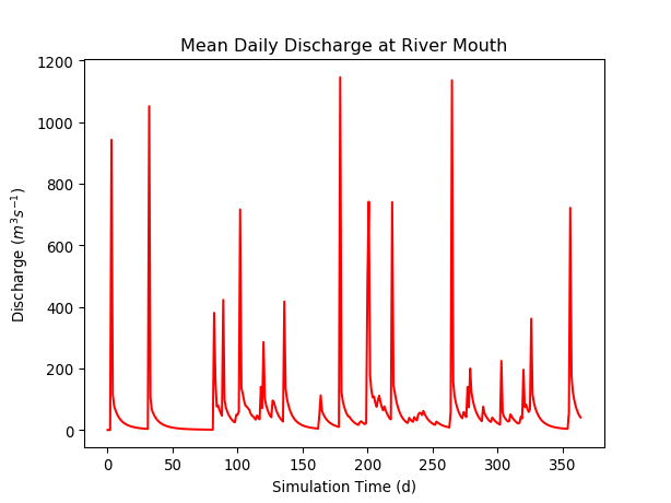
Let’s plot the daily mean water discharge values generated by the model. Start by importing Python’s matplotlib library, used for generating a variety of publication-quality figures:
>>> import matplotlib.pyplot as plt
Then set up a line plot of the discharge values:
>>> plt.plot(discharge, 'r')
Nothing appears on the screen yet; this statement only configures the plot. However, a plot isn’t complete until it has appropriate labels. Add some with:
>>> plt.title('Mean Daily Discharge at River Mouth')
>>> plt.xlabel('Simulation Time (d)')
>>> plt.ylabel('Discharge ($m^3 s^{-1}$)')
Now display the plot:
>>> plt.show()
A pair of more detailed Jupyter Notebook examples of using Hydrotrend can be found in the Examples section. An expanded description of the pymt methods used in this example can be found in the Usage section.